AI Anomaly Detection: Catch Issues Traditional Alerts Miss




Ready to get started?
Try OpenObserve Cloud today for more efficient and performant observability.
AI Anomaly Detection for Infrastructure & Applications: How It Works in 2026
Your database slows at 2:47 AM. By 3:15 AM, it's a full outage. The postmortem reveals the signal was there-disk I/O started behaving unusually around 1:00 AM-but no alert fired because there's no effective way to threshold "unusual I/O."
This is the gap ai anomaly detection fills. Instead of alerting when a metric crosses a predefined threshold (X > Y), ai anomaly detection alerts when a metric behaves differently than it historically has. Modern ai anomaly detection systems use machine learning to learn normal patterns from your data, then flag statistical deviations that indicate potential issues.
For DevOps and SRE teams managing complex distributed systems, ai anomaly detection has become essential infrastructure. Traditional threshold-based alerts miss gradual degradations, can't adapt to seasonal patterns, and generate alert fatigue through false positives. AI anomaly detection solves these problems by modeling expected behavior and surfacing truly unusual events.
This guide explores how ai anomaly detection works in observability contexts, the algorithms powering it, and how to implement it effectively for metrics, logs, and traces.
TL;DR: Key Takeaways on AI Anomaly Detection
- AI anomaly detection uses machine learning to identify unusual patterns in observability data without predefined thresholds
- Three algorithm families: Statistical baselines (z-score, IQR), time-series ML (Prophet, ARIMA), and tree-based models (Random Cut Forest, Isolation Forest)
- Three anomaly types: Metric anomalies (latency spikes, error rate surges), log anomalies (new error patterns), trace anomalies (slow spans)
- AI significantly reduces false positives compared to static thresholds by learning seasonal patterns and normal variance
- Key algorithms: Random Cut Forest (streaming data), Isolation Forest (batch detection), LSTM (complex seasonality)
- Implementation: Requires 3-7 days minimum training data, handles seasonality automatically, retrains periodically
- Real-world use cases: Kubernetes pod crashes, API latency degradation, LLM token cost spikes, security anomalies
AI anomaly detection is a core component of modern AIOps platforms, enabling AI-powered incident management that reduces mean time to resolution by providing early warning signals before threshold breaches occur.
What Is AI Anomaly Detection?
AI anomaly detection is the application of machine learning algorithms to automatically identify unusual patterns in time-series data, logs, and distributed traces. Unlike rule-based alerting that requires engineers to define what "bad" looks like upfront, AI anomaly detection learns what "normal" looks like from historical data and flags deviations.
The Core Problem: Unknown Unknowns
Traditional monitoring asks: "Is CPU above 80%?" AI anomaly detection asks: "Is CPU behaving differently than it ever has?"
This shift matters because:
- Gradual degradation goes unnoticed-latency drifting up 5ms per hour never crosses a threshold, but after 6 hours your service is down
- Seasonal baselines vary-1,000 errors/minute on Black Friday is normal; the same number at 4 AM Sunday indicates a crisis
- New failure modes emerge-you can't write thresholds for behaviors you haven't seen yet
How AI Anomaly Detection Works: The Basic Flow
Historical Data (7-30 days)
          ↓
   Training Phase (learn normal patterns)
          ↓
    Trained Model (encodes expected behavior)
          ↓
   New Data Point Arrives
          ↓
    Anomaly Score Calculation (how unusual is this?)
          ↓
   Score > Threshold? → Alert
The model continuously learns from new data, adapting to system changes while maintaining the ability to detect true anomalies.
Why Static Thresholds Break
Most alerting systems rely on static thresholds: "Alert when error rate > 100/min" or "Alert when latency > 500ms." This approach fails in three critical ways:
1. Context Blindness
A static threshold doesn't know that:
- 200 errors during a Monday morning deployment rush is noise
- 200 errors at 4 AM Saturday is a critical incident
- CPU at 70% is normal during batch processing, alarming during off-hours
2. Threshold Tuning Fatigue
Finding the "right" threshold is impossible:
- Too low: Alert storms and fatigue (the boy who cried wolf)
- Too high: Miss incidents until customer impact
- Just right: Lasts a week until traffic patterns change
3. No Adaptation to Change
Your system evolves:
- New features shift normal behavior
- Traffic grows 3× over 6 months
- Deployment frequency doubles
Static thresholds don't adapt-they require constant manual tuning or become obsolete.
AI Anomaly Detection Algorithms: How They Work
Multiple algorithmic approaches power AI anomaly detection, each with different trade-offs for observability use cases.
1. Statistical Baseline Methods
Approach: Calculate statistical properties (mean, standard deviation, percentiles) from historical data and flag points that deviate significantly.
Common Techniques:
Z-Score (Standard Score)
z = (x - μ) / σ

Where:
x = current value
μ = historical mean
σ = historical standard deviation

Flag if |z| > 3 (point is 3+ standard deviations from mean)
Pros: Simple, fast, interpretable Cons: Assumes normal distribution, can't handle seasonality, sensitive to outliers
Interquartile Range (IQR)
IQR = Q3 - Q1 (75th percentile - 25th percentile)
Flag if: x < Q1 - 1.5×IQR  OR  x > Q3 + 1.5×IQR
Pros: Robust to outliers, no distribution assumptions Cons: Still can't handle seasonality or trends
When to use: Quick detection on stable metrics without strong patterns (e.g., cache hit rates, connection pool sizes)
2. Time-Series Forecasting Models
Approach: Build predictive models that forecast expected values with confidence intervals. Flag points that fall outside the predicted range.
Prophet (Facebook's Algorithm)
Decomposes time series into:
- Trend: Long-term increase/decrease
- Seasonality: Daily, weekly, yearly patterns
- Holidays/Events: Known special dates
- Residuals: Everything else (noise + anomalies)
y(t) = trend(t) + seasonality(t) + holidays(t) + error(t)
Pros: Handles multiple seasonalities automatically, interpretable components, robust to missing data Cons: Requires longer training windows (weeks), computationally expensive, batch-oriented
ARIMA (AutoRegressive Integrated Moving Average)
Statistical model using past values and past errors to predict future:
ARIMA(p, d, q)
p = autoregressive terms (use past p values)
d = differencing to remove trends
q = moving average terms (use past q errors)
Pros: Strong theoretical foundation, handles trends and seasonality Cons: Requires stationary data, parameter tuning complex, doesn't scale to high-cardinality
When to use: Metrics with strong daily/weekly patterns (API request rates, user activity), business metrics with known seasonality
3. Tree-Based Isolation Methods
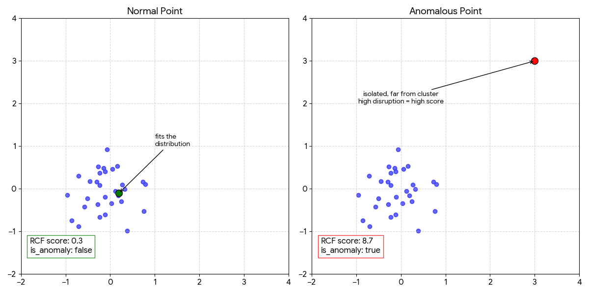
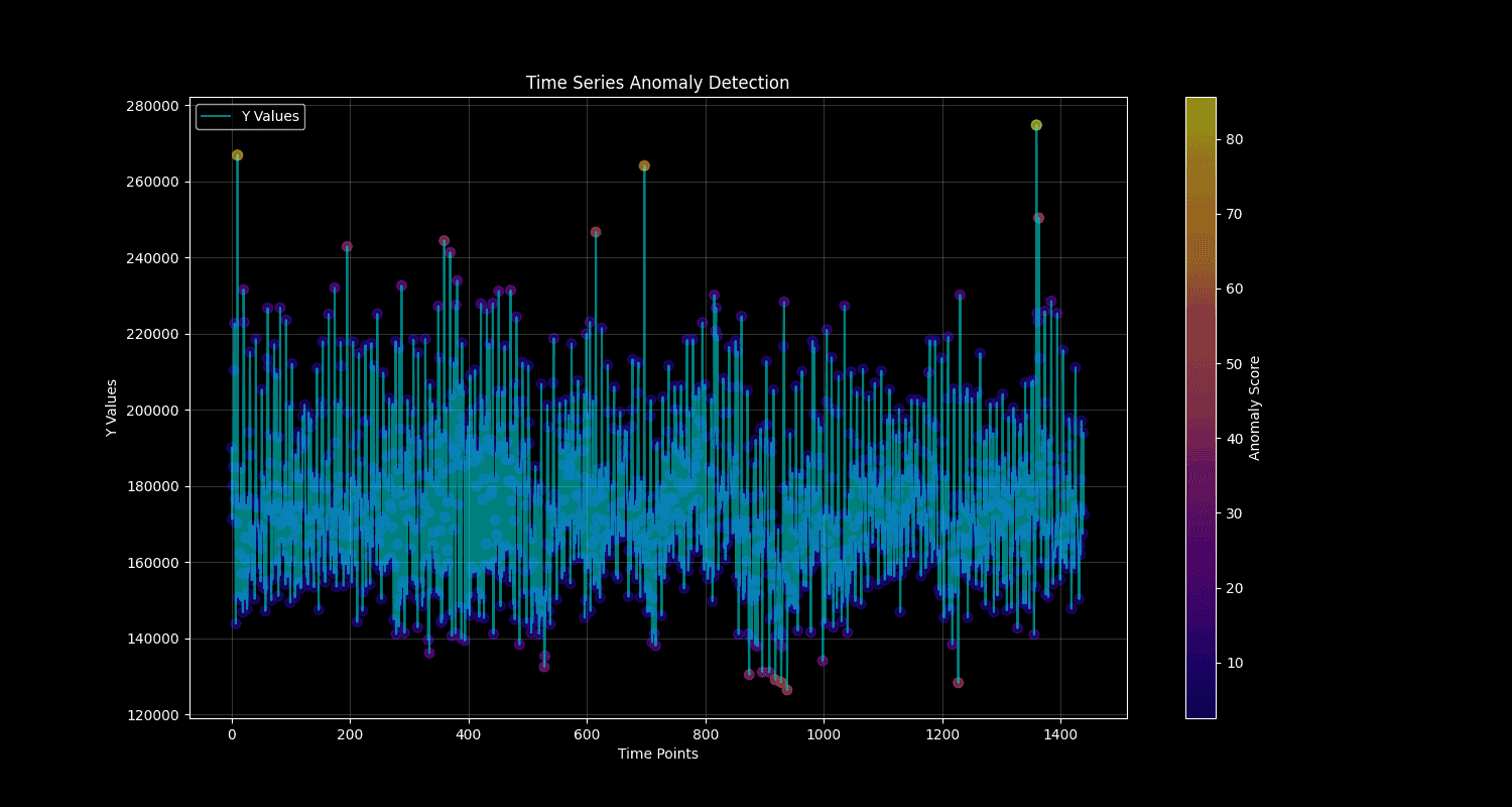
Approach: Build decision trees that isolate anomalies through recursive partitioning. Anomalies are easier to isolate (require fewer splits) than normal points.
Isolation Forest
Creates random binary trees by:
- Randomly selecting a feature and split value
- Partitioning data recursively
- Anomalies end up in shorter tree paths (isolated quickly)
Anomaly Score = 2^(-average_path_length / normalization_factor)

High score = short path = anomaly
Low score = long path = normal
Pros: Unsupervised (no labels needed), handles high dimensions, fast inference Cons: Batch-oriented (not streaming), sensitive to feature scaling
Random Cut Forest (Amazon's RCF)
Streaming version of Isolation Forest optimized for time-series:
- Processes data points sequentially as they arrive
- Maintains a sliding window of recent data
- Uses shingle size (sliding window of consecutive values) for context
Shingle Size = 8 example:
Data:  [42, 45, 43, 44, 46, 44, 45, 91]
                                   ↑
                Score this value in context of 7 preceding values
                Sudden jump after flat baseline → high score
Pros: Streaming-native, handles seasonality via shingling, explainable scores, no labeled data Cons: More complex to tune, requires understanding shingle size/threshold trade-offs
When to use: High-velocity streaming data (logs, metrics from Kubernetes), time-series where context matters (gradual drift detection)
4. Neural Network Approaches
LSTM (Long Short-Term Memory) Autoencoders
Neural networks that:
- Encode time-series into compressed representation
- Decode back to reconstruct original series
- Reconstruction error indicates anomaly (can't reconstruct unusual patterns)
Training: Normal data → minimize reconstruction error
Detection: New data → large reconstruction error = anomaly
Pros: Learns complex patterns, handles multivariate data, no explicit feature engineering Cons: Requires large datasets, black-box (not explainable), expensive training, GPU often needed
When to use: Complex multivariate signals (correlated metrics across services), sufficient training data (months), tolerance for higher operational cost
Types of Anomalies in Observability
AI anomaly detection applies differently across metrics, logs, and traces-each requiring distinct approaches.
Metric Anomalies: Time-Series Deviations
What: Numerical measurements collected at regular intervals (CPU, memory, request rates, latency percentiles)
Detection Approach: Time-series forecasting or streaming tree models
Common Anomaly Patterns:
1. Point Anomalies (Spikes/Dips)
- Single data point drastically different from neighbors
- Example: Latency spike from 50ms → 2,000ms for one minute
- Detection: Any algorithm works; easiest to catch
2. Contextual Anomalies
- Value normal in one context, anomalous in another
- Example: 10,000 requests/min at 2 PM = normal; same at 3 AM = DDoS or runaway retry
- Detection: Requires seasonality awareness (Prophet, RCF with weekly training)
3. Trend Anomalies (Drift)
- Gradual shift in baseline behavior
- Example: Memory consumption increasing 2% per hour (leak)
- Detection: ARIMA, Prophet, RCF with large shingle size
Example: API Latency Spike Detection
Metric: api_latency_p99_ms
Historical baseline: 45ms ± 8ms (weekday afternoons)
New observation: 180ms

Z-score: (180 - 45) / 8 = 16.8 → Strong anomaly
RCF score: 12.4 (threshold: 97th percentile ≈ score 3.0) → Alert
Log Anomalies: Pattern Deviations
What: Unstructured or semi-structured text events (application logs, system logs, audit logs)
Detection Approach: Text clustering + frequency analysis
Common Techniques:
1. Log Template Extraction
- Parse logs into templates by replacing variables
- Example:
"User 12345 logged in from 192.168.1.100"→"User <ID> logged in from <IP>" - Count occurrences of each template over time
2. Clustering-Based Anomaly Detection
- Use NLP embeddings (BERT, sentence transformers) to vectorize log messages
- Cluster similar messages
- New messages that don't fit any cluster = anomalies
3. Frequency-Based Detection
- Track count of each log pattern
- Apply time-series anomaly detection to pattern counts
- Example: "Database connection timeout" appears 200× more than baseline → alert
Example: New Error Pattern
Historical: 0 occurrences of "OutOfMemoryError: GC overhead limit exceeded"
New: 47 occurrences in last 5 minutes

Simple frequency: 47 vs baseline 0 → anomaly
ML clustering: Message doesn't match any known cluster → anomaly
Trace Anomalies: Distributed Request Deviations
What: End-to-end request flows through distributed services (spans with timing, dependencies, errors)
Detection Approach: Span duration analysis + dependency graph anomalies
Common Patterns:
1. Slow Spans
- Individual service call taking longer than expected
- Example: Database query span normally 15ms, now 800ms
- Detection: Time-series anomaly on span duration distribution
2. New Error Paths
- Error appearing in previously healthy span
- Example:
payment-service → bank-apispan starts returning 503s - Detection: Error rate anomaly per service pair
3. Topology Anomalies
- New or missing service dependencies
- Example:
checkout-servicesuddenly callinglegacy-billing-apinot seen in 6 months - Detection: Graph analysis on service call patterns
Example: Database Degradation via Traces
Span: inventory-service → postgres (SELECT query)
Historical p95 duration: 35ms
Recent 10 minutes p95: 250ms

RCF anomaly score: 8.7 → Flag as anomaly
Alert: "Database query latency anomaly detected 20 minutes before error rate spike"
AI vs Traditional Threshold Alerting: The Comparison
| Dimension | Static Thresholds | AI Anomaly Detection |
|---|---|---|
| Setup effort | 5 minutes (set threshold) | 3-7 days training + tuning |
| Adaptation | Manual updates required | Automatic with retraining |
| False positive rate | Higher in dynamic environments | Lower with proper tuning |
| Seasonal handling | Requires multiple thresholds | Learned automatically |
| Gradual drift detection | Misses completely | Catches via shingle/context |
| Unknown failure modes | Can't detect | Can flag unusual patterns |
| Explainability | Perfect ("CPU > 80%") | Moderate (score + deviation %) |
| Computational cost | Negligible | Model training + inference |
When to Use Each Approach
Use static thresholds when:
- Failure condition is absolute (disk > 95% always bad)
- You need zero false negatives (security: this error must never occur)
- You have < 3 days of data (not enough to train)
- Metric is highly stable (cache hit rate on read-heavy workload)
Use AI anomaly detection when:
- Metric has strong patterns (hourly/daily/weekly seasonality)
- Normal ranges vary by time of day, day of week
- You want early warning (detect before threshold breach)
- Exploration mode (find issues you don't know to look for)
Use both together:
- Static threshold: disk > 90% (hard limit)
- AI anomaly: disk filling rate faster than historical baseline (early warning)
Real-World Use Cases
1. Kubernetes Pod Crash Anomalies
Scenario: Detecting unusual pod restart rates before they cascade into outages
Implementation:
Metric: pod_restarts_per_5min (by namespace, deployment)
Algorithm: Random Cut Forest
Training window: 14 days
Threshold: 97th percentile

Normal baseline: 0-2 restarts per 5 min
Anomaly trigger: 8 restarts in 5 min at 3 AM
Outcome: Alert fires 15 minutes before memory leak causes cascading pod failures across deployment
2. API Latency Degradation
Scenario: Gradual database slowdown that never crosses absolute threshold
Implementation:
Metric: api_latency_p99_ms
Algorithm: Prophet (handles daily patterns)
Training window: 30 days
Confidence interval: 95%

Normal: 45ms ± 12ms (2 PM weekday)
Detection: Latency drifting 2ms/hour over 6 hours
At hour 6: 57ms (still under 100ms threshold, but 3σ from forecast)
Outcome: DBA investigates, finds query plan regression from index change 6 hours prior-reverts before customer impact
3. Error Rate Surge in Logs
Scenario: New error pattern appearing after deployment
Implementation:
Data: Application error logs
Algorithm: Log clustering + frequency anomaly
Training: 7 days of log templates

New pattern: "NullPointerException in PaymentProcessor.validateCard()"
Historical frequency: 0 occurrences
New frequency: 127 in 10 minutes
Outcome: Rollback initiated automatically, deployment rolled back before affecting 5% of users
4. LLM Token Cost Anomalies
Scenario: Detecting runaway LLM API costs from prompt injection or inefficient calls
Implementation:
Metric: llm_tokens_used_per_hour (by service, model)
Algorithm: IQR (handles cost spikes)
Training window: 21 days

Normal: 50K-80K tokens/hour (GPT-4)
Anomaly: 450K tokens/hour at 2 AM
Outcome: Alert fires, investigation reveals infinite retry loop in summarization service, circuit breaker engaged
5. Security: Unusual User Behavior
Scenario: Detecting compromised account via unusual access patterns
Implementation:
Metric: api_calls_per_user_per_hour
Algorithm: Isolation Forest (multivariate)
Features: [call_count, unique_endpoints, failed_auth_attempts, geographic_distance]

Normal user: 20-40 calls/hour, 3-5 endpoints, 0 failed auth, same region
Anomalous: 800 calls/hour, 45 endpoints, 12 failed auth, new country
Outcome: Account flagged, MFA challenge triggered, investigation reveals credential stuffing attack
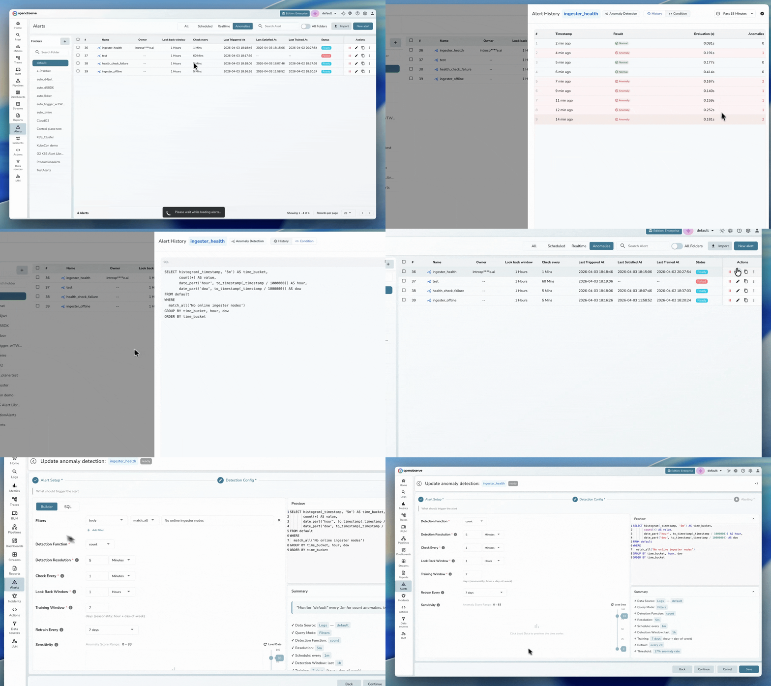
OpenObserve's Anomaly Detection: Built-In Rust-Powered Engine
OpenObserve ships with a production-ready anomaly detection engine powered by Random Cut Forest (RCF)-the same algorithm Amazon uses in Kinesis Data Analytics.
Why Random Cut Forest?
| Requirement | RCF Solution |
|---|---|
| Streaming data | Processes points sequentially as they arrive |
| No labeled data | Fully unsupervised learning |
| Handles seasonality | Shingle size + training window capture patterns |
| Fast inference | 5-second detection runs on 100+ concurrent jobs |
| Explainable | Anomaly scores with deviation percentages |
Architecture: Rust for Scale
When 50 detection jobs fire every 30 minutes-each loading a model from S3 and scoring hundreds of points-runtime performance matters:
- No garbage collection pauses that corrupt timing windows
- Compile-time thread safety for concurrent job execution
- Precise memory management (100-tree RCF forest = 2-5 MB, no heap bloat)
Performance (in our testing on 16-core servers):
- Training 30 days of 5-minute data (~8,640 points): < 60 seconds
- Detection scoring per run: < 5 seconds
- Concurrent jobs: 50+ without resource contention
The model learns that Monday 9 AM has 2× the latency of Saturday 4 AM. A 200ms spike on Monday morning is noise; the same spike at 4 AM Saturday fires immediately-without defining any of that logic.
By combining intelligent anomaly detection with automated alert correlation, teams can reduce mean time to resolution significantly-catching issues before they escalate to customer-facing incidents.
Want the full technical deep-dive? See our complete implementation guide: Real-Time Anomaly Detection with OpenObserve and Random Cut Forest
Key Capabilities
1. Automatic Seasonality Detection
Training window → Seasonality learned
1-6 days        → Daily (24-hour cycles)
7+ days         → Weekly (daily + weekday/weekend patterns)
2. Model Retraining
- Default: Retrain every 7 days automatically
- Manual trigger via API for immediate baseline updates post-deployment
- Version tracking: Every anomaly records which model version scored it
3. Full Auditability
-- Query all anomalies from last 24 hours
SELECT anomaly_name, actual_value, deviation_percent,
       score, _timestamp
FROM "_anomalies"
WHERE is_anomaly = true
  AND _timestamp > now() - interval '24 hours'
ORDER BY score DESC
4. Tuning Controls
- Threshold (90-99): Higher = only extreme outliers
- Shingle size (4-16): Larger = more context, catches gradual drift
- Training window (7-90 days): Longer = more pattern history
- Detection window: How far back each run scores
AI Anomaly Detection Platforms: 2026 Comparison
Multiple platforms offer AI-powered anomaly detection with different strengths and trade-offs. Here's how leading solutions compare:
Platform Capabilities Comparison
| Platform | Algorithm Approach | Streaming Support | Custom Queries | Best For |
|---|---|---|---|---|
| OpenObserve | Random Cut Forest (RCF) | Native streaming | Full SQL flexibility | Cost-sensitive teams, custom aggregations, full control |
| Datadog | Proprietary ensemble | Yes | Limited to predefined metrics | Teams already on Datadog APM/infra |
| AWS CloudWatch | Random Cut Forest | Yes | CloudWatch Metrics only | AWS-native infrastructure |
| New Relic | ML ensemble | Yes | NRQL queries | Full-stack observability users |
| Grafana ML | Prophet + seasonal decomp | Batch-oriented | PromQL/Flux queries | Budget-conscious, existing Grafana users |
| Dynatrace | Davis AI (proprietary) | Yes | Limited | Enterprise, auto-instrumentation |
Datadog Anomaly Detection: Detailed Comparison
Datadog offers anomaly detection as part of its monitoring platform. Here's how the technical approach compares:
Algorithm Comparison
| Feature | OpenObserve (RCF) | Datadog |
|---|---|---|
| Algorithm | Random Cut Forest (Amazon RCF) | Proprietary (likely ensemble of methods) |
| Streaming | Yes (native) | Yes |
| Seasonality | Auto-detected (daily/weekly) | Auto-detected (configurable) |
| Training data | 7-90 days | 1-4 weeks (recommended) |
| Retraining | Auto every 7 days (configurable) | Continuous sliding window |
| Custom SQL | Yes (any aggregation) | No (predefined metrics only) |
| Explainability | Score + deviation % + model version | Bounds visualization |
Cost Model Differences
Datadog:
- Anomaly detection included in monitoring plans (no separate SKU)
- Costs scale with metric cardinality and custom metrics
- High-cardinality metrics (Kubernetes labels, container IDs) can significantly increase costs
OpenObserve:
- Anomaly detection included in Enterprise plan
- No per-metric pricing-unlimited anomaly detection configs
- Storage-based pricing with columnar compression (Parquet)
Cost Advantage: OpenObserve's architecture enables significantly lower costs at scale for teams running many anomaly detection configs, particularly with high-cardinality data.
Feature Differences
Datadog Advantages:
- Tighter integration with Datadog APM/infrastructure UI
- Anomaly detection on derived metrics (ratios, formulas) without custom queries
- Mobile app notifications
OpenObserve Advantages:
- Custom SQL flexibility: Anomaly detection on any aggregation (percentiles, custom window functions)
- Full data access: Query
_anomaliesstream directly for analysis - Model control: Manual retraining, version tracking, threshold tuning per config
- Open architecture: Export models, integrate with external alerting
Common Pitfalls & How to Avoid Them
Real-world lessons from DevOps and SRE practitioners implementing AI anomaly detection:
Pitfall 1: Training on Incident Windows
Problem: "We trained our model on 30 days of data that included a major outage. Now it thinks 50% error rates are normal." - Reddit r/devops
Why it happens: Models learn from all training data-if that includes anomalies, they become part of the baseline.
Solution:
- Exclude known incident time ranges from training data
- Use status page data to filter out degraded periods
- Start with a clean baseline after system stabilizes post-incident
Pitfall 2: Ignoring Deployment-Induced Baseline Shifts
Problem: "Every deployment triggers 20+ false positive alerts for 2 hours until things stabilize." - HackerNews discussion
Why it happens: Deployments often change performance characteristics (new caching, query optimizations, feature flags). Models trained on pre-deployment data flag the new normal as anomalous.
Solution:
- Trigger manual retraining immediately after major deployments
- Use temporary threshold increases (97 → 99) during deployment windows
- Implement blue-green deployments to compare new vs old baselines
- Set
retrain_interval_daysto match your deployment frequency
Pitfall 3: Over-Tuning on Historical Data
Problem: "Our model is tuned perfectly on last month's data but misses new failure modes completely." - Reddit r/sre
Why it happens: Overfitting to past patterns reduces sensitivity to novel anomalies.
Solution:
- Keep thresholds conservative (95-97, not 99+)
- Maintain a validation set from recent weeks (don't train on ALL data)
- Monitor "score distribution" over time-scores should vary, not cluster tightly
- Combine with static thresholds for known-bad absolute values
Pitfall 4: Insufficient Training Data for Seasonal Patterns
Problem: "We trained on 7 days of data. Every Monday morning triggers false alerts because the model never saw Monday load."
Why it happens: Weekly seasonality requires at least 2-3 full weeks to learn weekday vs. weekend patterns.
Solution:
Training window guidelines:
- Daily patterns only: 7-14 days minimum
- Weekly patterns (weekday/weekend): 21-30 days minimum
- Monthly patterns: 60-90 days minimum

Rule: Training window ≥ 3× your strongest seasonal cycle
Pitfall 5: Alert Fatigue from Low-Impact Anomalies
Problem: "We get 50 anomaly alerts per day. Team started ignoring them after week 1." - DevOps practitioner
Why it happens: Not all anomalies require immediate action. Low-severity anomalies mixed with critical ones create noise.
Solution:
- Route alerts based on anomaly score:
- Score > 10: Page on-call (immediate action)
- Score 5-10: Slack channel (review within 1 hour)
- Score 3-5: Log only (weekly review)
- Add business impact filters: Only alert on customer-facing services
- Combine with error rate thresholds: Anomaly + error rate > X = page
Pitfall 6: Not Monitoring Model Performance
Problem: "Our 6-month-old model stopped catching real incidents. We didn't notice for weeks."
Why it happens: Model drift-as systems evolve, old models become less relevant.
Solution:
- Track model age in dashboards
- Monitor anomaly detection rate over time (should be ~3-5% of points)
- Set alerts on model staleness (> 30 days without retrain)
- Review postmortems: Did anomaly detection fire? When? Score?
Take the Next Step
AI anomaly detection transforms how DevOps and SRE teams handle incident response-catching issues traditional thresholds miss, reducing alert fatigue, and adapting automatically as systems evolve.
As a core component of modern AIOps platforms, AI anomaly detection enables proactive incident management that reduces MTTR by providing early warning signals 20-40 minutes before customer-facing impact.
For teams managing Kubernetes, microservices, or any system with seasonal traffic patterns, AI anomaly detection isn't optional anymore-it's how you stay ahead of incidents instead of reacting to them.
Ready to implement AI anomaly detection?
- Deep dive: Real-Time Anomaly Detection with OpenObserve and Random Cut Forest
- Get started: Sign up for OpenObserve Cloud (14-day free trial, anomaly detection included)
- Self-host: Download OpenObserve for on-prem deployment
- Learn more: OpenObserve Documentation
Questions? Join our community: OpenObserve Slack • GitHub
Frequently Asked Questions
About the Author
Manas Sharma


Manas is a passionate Dev and Cloud Advocate with a strong focus on cloud-native technologies, including observability, cloud, kubernetes, and opensource. building bridges between tech and community.
Follow OpenObserve on Google
Add OpenObserve as a preferred source to see more of our articles in Google Search and Top Stories.