Catch Anomalies Before They Become Incidents: Inside OpenObserve's Built-In Detection Engine





Ready to get started?
Try OpenObserve Cloud today for more efficient and performant observability.

Your database slows at 2:47am. By 3:15am it's a full outage. The postmortem shows the signal was there — disk I/O started behaving unusually around 1am — but no alert fired because there's no good way to threshold "unusual I/O."
This is the gap anomaly detection fills. Not "alert when X > Y" — but "alert when X is behaving differently than it historically has."
OpenObserve ships a built-in anomaly detection engine powered by Rust and Random Cut Forest. Point it at a stream, set a training window, and it learns what normal looks like for your data — then alerts when things stop looking normal. No external scripts. No ML infrastructure. No labeled training data.
Already read our API-based anomaly detection guide? This is about the engine built into OpenObserve — same algorithm, zero setup overhead.
Why Static Thresholds Break
Most alerting asks you to define what "bad" looks like upfront. That works until it doesn't:
- Gradual degradation — latency drifting up 5ms/hour never crosses a threshold, but after 6 hours you're down
- Seasonal baselines — 1,000 errors/min on Black Friday is fine; the same number at 4am Sunday is a crisis
- Unknown unknowns — what should disk I/O look like at 1am on a Tuesday?
OpenObserve's approach: train a model on your historical data, then score new data against what the model expects.
Random Cut Forest: The Algorithm
OpenObserve uses Random Cut Forest (RCF) — Amazon's algorithm powering Kinesis Data Analytics anomaly detection. It's the right choice for observability data:
| Approach | No labels needed | Handles seasonality | Streaming-native | Explainable |
|---|---|---|---|---|
| Static threshold | — | No | Yes | Yes |
| Z-score / IQR | Yes | No | Yes | Partial |
| Isolation Forest | Yes | Partial | No | Partial |
| LSTM (neural net) | No | Yes | No | No |
| Random Cut Forest | Yes | Yes | Yes | Yes |
How scoring works
RCF builds a forest of 100 random decision trees on your historical time series. Each tree encodes the "shape" of normal behavior. When a new point arrives, the algorithm measures how far it would need to travel to change the forest's partition structure — that's the anomaly score.
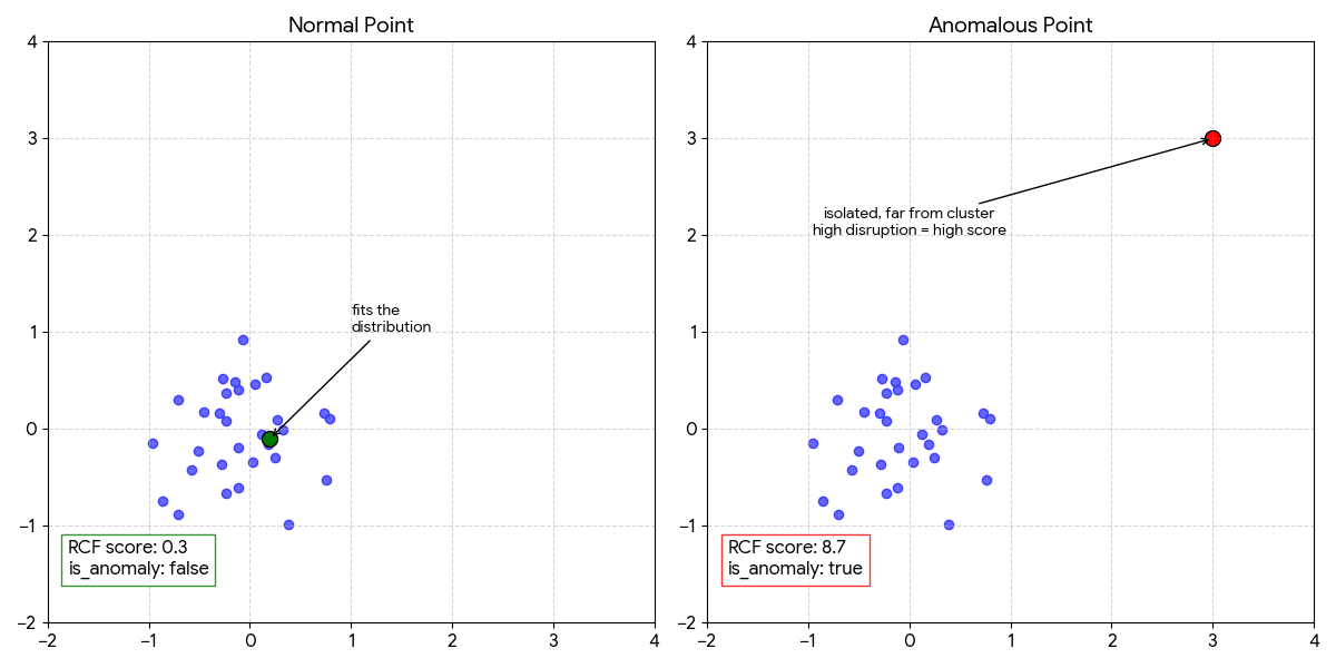
When a score exceeds the Nth percentile of training scores, the point is flagged. Default is 97th percentile top 3% of unusual behavior.
Shingle size: scoring with context
RCF scores a sliding window of consecutive values together (shingle size), not individual points. With shingle size 8:
Data:   [42, 45, 43, 44, 46, 44, 45, 91]
                                      ↑
                           This value scored in context
                           of the 7 values before it.
                           A sudden jump after a flat
                           baseline = high score.
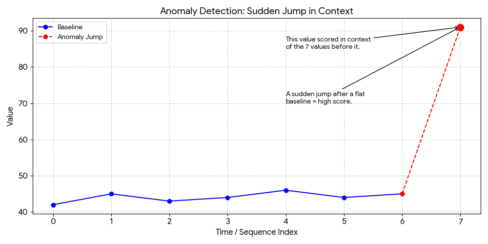
This catches what point-based approaches miss: gradual drifts, pattern breaks, and contextual anomalies (normal at 2pm, unusual at 2am).
The Detection Pipeline
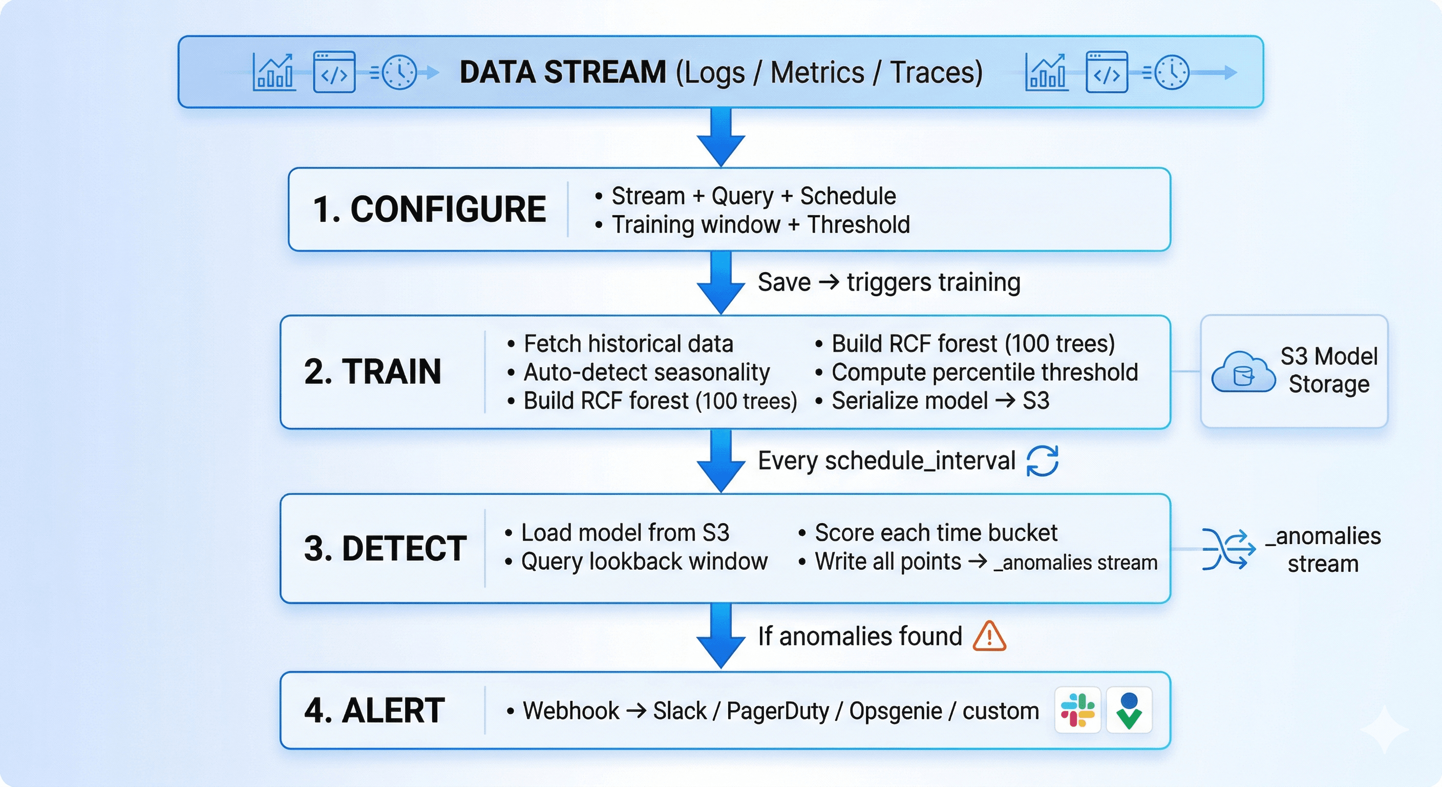
Seasonality is auto-detected at training time based on how much history exists:
| Training window | Seasonality | What it learns |
|---|---|---|
| 1–6 days | Day | Hour-of-day patterns (24-hour daily cycles) |
| 7+ days | Week | Hour-of-day + day-of-week (weekday vs. weekend) |
The feature vector fed to RCF expands with seasonality: [value] → [value, hour/24] → [value, hour/24, dow/7]. The model and its feature space are locked at training time, so detection always uses the exact same dimensionality the model was trained on.
Each scored point written to _anomalies carries: _timestamp, actual_value, score, threshold_value, is_anomaly, deviation_percent, model_version. The last_processed_timestamp is tracked per config — no double-counting between runs.
Why Rust Powers This at Scale
When 50 detection jobs fire every 30 minutes — each loading a model from S3 and scoring hundreds of data points — the runtime choices matter.
- No GC pauses — GC pauses in Java/Go engines corrupt timing-sensitive detection windows. Rust has no GC.
- Compile-time thread safety — jobs run concurrently. Rust eliminates data races at compile time, not at runtime.
- Precise memory — a 100-tree RCF forest deserializes to exactly what it needs. No heap bloat across long-running processes.
In practice: Training 30 days of 5-minute bucket data (~8,640 points) completes in under 60 seconds. Each detection run scores a window in under 5 seconds. The model itself is 2–5 MB on S3.
Real-World Examples
Error rate spikes in application logs
Stream:             app-logs           (Logs)
Filter:             level = "error"
Detection function: count(*)
Histogram interval: 5m
Schedule interval:  30m
Detection window:   1800s
Training window:    14 days
Threshold:          97
RCF learns that Monday 9am has 3× the error volume of Saturday 4am. 200 errors on Monday morning is noise. The same 200 errors at 4am Saturday fires immediately — without you defining any of that logic.
API latency degradation in metrics
-- Custom SQL for p99 latency per 5-minute bucket
SELECT
  date_bin('5 minutes', _timestamp, '1970-01-01') AS _timestamp,
  percentile_cont(0.99) WITHIN GROUP (ORDER BY response_time_ms) AS value
FROM "infra-metrics"
WHERE service = 'payments-api'
  AND _timestamp BETWEEN {start_time} AND {end_time}
GROUP BY 1
ORDER BY 1
Training window:  30 days     Threshold: 99
Schedule:         15m         Detection window: 3600s
The shingle window catches gradual drift — latency climbing 2ms/hour over a day — before it becomes visible to any static threshold or human reviewer.
Slow spans in distributed traces
Stream:    traces    Filter: service.name = "inventory-service" AND duration > 500ms
Function:  count(*)  Histogram: 10m   Training: 21 days   Threshold: 97
Catches database degradation via slow span count increases — typically 20–30 minutes before the service starts returning errors.
Disk filling faster than normal
SELECT date_bin('1 hour', _timestamp, '1970-01-01') AS _timestamp,
       avg(disk_used_percent) AS value
FROM "host-metrics"
WHERE host = 'prod-db-01'
  AND _timestamp BETWEEN {start_time} AND {end_time}
GROUP BY 1 ORDER BY 1
Training window:  60 days (→ weekly seasonality)   Threshold: 95
Schedule:         6h                                Detection window: 21600s
RCF learns the normal growth rate. It fires when disk is filling 3× faster than historical norms — hours before any percentage threshold would trigger.
Tuning Reference
Threshold
| Value | Behavior | Use when |
|---|---|---|
| 90–94 | Catches subtle deviations, more noise | Security monitoring, exploratory |
| 95–97 (default) | Balanced | General production monitoring |
| 98–99 | Extreme outliers only | Payments, auth — low false-positive tolerance |
Start at 97. Too noisy → raise to 99. Missing incidents → lower to 95.
Training window and histogram interval
| Signal type | Training window | Histogram interval |
|---|---|---|
| App errors | 14 days | 1m–5m |
| API latency (p99) | 30 days | 5m–15m |
| Infrastructure metrics | 30–60 days | 15m–1h |
| Business metrics | 60–90 days | 1h–1d |
Detection window formula
detection_window_seconds = schedule_interval_seconds × 2
Always overlap — ensures no gap between runs if a run is slightly delayed.
Anomaly Scores at a Glance
| Score | Interpretation |
|---|---|
| < 1.0 | Normal |
| 1.0–2.0 | Slightly unusual |
| 2.0–5.0 | Notable — investigate if persistent |
| > 5.0 | Strong anomaly |
| > 10.0 | Extreme — act immediately |
deviation_percent is often more useful for stakeholder communication than the raw score.
Model Retraining
Models trained on last month's data drift out of relevance as systems evolve. OpenObserve retrains automatically via retrain_interval_days (default: 7).
Every 7 days: fresh training data → new versioned RCF forest → S3 → seamless switch on next detection run. The most recent model versions are retained — _anomalies records the model_version that scored each point, making it straightforward to investigate if retraining changed sensitivity.
Set retrain_interval_days = 0 to lock the baseline permanently.
After a deployment that shifts your metric significantly: don't wait 7 days. Force a retrain immediately:
curl -X POST \
  "https://your-openobserve.example.com/api/{org}/anomaly_detection/{id}/train" \
  -H "Authorization: Basic ..."
Querying the _anomalies Stream
Every scored point — anomalous or not — lands here. Query it directly in OpenObserve:
-- All anomalies in the last 24 hours, worst first
SELECT anomaly_name, actual_value, deviation_percent, score, _timestamp
FROM "_anomalies"
WHERE is_anomaly = true AND _timestamp > now() - interval '24 hours'
ORDER BY score DESC

-- Which configs are most noisy this week?
SELECT anomaly_name, count(*) as alerts
FROM "_anomalies"
WHERE is_anomaly = true AND _timestamp > now() - interval '7 days'
GROUP BY anomaly_name ORDER BY alerts DESC

-- Score distribution — helps decide if threshold needs adjusting
SELECT
  CASE WHEN score < 1.0 THEN 'normal'
       WHEN score < 2.0 THEN 'slight'
       WHEN score < 5.0 THEN 'notable'
       ELSE 'strong' END AS band,
  count(*) AS n
FROM "_anomalies"
WHERE anomaly_id = 'your-id' AND _timestamp > now() - interval '30 days'
GROUP BY 1 ORDER BY 2 DESC
Troubleshooting
| Symptom | Fix |
|---|---|
| Status: Failed immediately | Query returns no data — check stream name, filters, training window length |
| Too many false positives | Raise threshold (97 → 99), widen training window, coarsen histogram interval |
| Missing real incidents | Lower threshold (97 → 95), reduce histogram interval |
is_anomaly always false |
Your system is highly consistent (good!) — or lower threshold to 90 to verify scoring is running |
| False positives after deploy | Expected. Trigger manual retrain or wait for next auto-retrain cycle |
When NOT to Use It
Anomaly detection and static alerts are complementary, not interchangeable. Use a static alert when:
- The bad value is absolute —
disk > 90%is always bad regardless of history - You need a guarantee, not a probability — "this error must never occur"
- You have < 3 days of data — RCF has nothing to learn from
- Frequent deployments constantly shift the baseline — the model can't keep up between retraining cycles
Getting Started
Prerequisites: OpenObserve Enterprise · a stream with data · an alert destination configured
UI (quickest path)
- Alerts → Anomaly Detection → Add Anomaly Detection
- Step 1: Name + stream type + stream
- Step 2: Filter or custom SQL · histogram
5m· schedule30m· training window14days - Step 3: Enable alerting · pick destination
- Save → training starts automatically
Status goes: Training → Waiting → detection runs on schedule.
Summary
Static alerts tell you when something crossed a line you drew. Anomaly detection tells you when something is behaving differently than it ever has — which is usually the earlier, more useful signal.
OpenObserve's engine gives you:
- No ML infrastructure — training, scheduling, model versioning, and alerting are fully managed
- Any data type — logs, metrics, traces, or custom SQL aggregates
- Automatic seasonality — learns daily/weekly patterns without configuration
- Rust performance — concurrent jobs, no GC pauses, 5-second detection runs
- Full auditability — every scored point in
_anomalies, queryable and dashboardable
Pick the one stream you have the least visibility into. Set a 14-day training window. Run it for a week. You'll be surprised what it finds.
FAQ
Do I need labeled anomaly examples?
No ,RCF is fully unsupervised.
What if I have less than 7 days of data?
Set training_window_days to 1–3 and increase as data accumulates. Early results will be rough.
Can custom SQL join multiple streams?
Not currently, queries must target a single stream.
Does this work with Prometheus metrics?
Yes ,any numeric field in any OpenObserve stream works.
Questions? OpenObserve Slack · GitHub
About the Authors
Bhargav Patel

Bhargav Patel is a frontend-focused Software Engineer working on observability platforms. He builds seamless user experiences for visualizing and interacting with system data like logs, metrics, and traces. His focus is on performance, usability, and developer experience.
Loakesh Indiran
Loakesh is a passionate engineer and open-source contributor focused on building distributed & scalable systems and developer tools. He works across databases, distributed systems, cloud-native technologies, observability, actively contributing to projects like OpenObserve, Apache Datafusion while building impactful products.